The dashboard told me that 30,000 training iterations had produced a worse result than 7,000. It was wrong. I had captured the score of one arbitrary held-out frame instead of the test-set mean.
That mistake became the most useful result from exercising ReconStudio, the browser workflow, job API and experiment ledger I built around a Gaussian splat pipeline. The application made it easier to run the pipeline. Using it repeatedly showed me which evidence I could trust.
The ledger contains 24 job records across six scenes. Seventeen completed, six failed, and one was abandoned while still marked as running. Fifteen distinct runs are documented in my notes; the others were repeats and early probes. The set includes benchmark photographs, a phone video, a multi-camera dataset that I configured incorrectly, Gaussian budgets from one to four million, and short and full training runs.
This was an iterative build, not a balanced benchmark study. I changed the application and its metric collection while I was learning. That makes the failed jobs useful engineering evidence, but it limits the claims I can make about reconstruction quality. Comparing the same scene and held-out frames controls for frame difficulty. It does not isolate one trainer setting when the complete camera solve and training run are repeated.

The setup behind the numbers
These measurements came from one machine and one software configuration:
| Component | Tested configuration |
|---|---|
| Compute | AWS EC2 g6e.2xlarge |
| GPU | One NVIDIA L40S, 48 GB GDDR6 ECC, 46,068 MiB usable |
| CPU and memory | 8 vCPUs and 64 GiB RAM |
| Host | Ubuntu 24.04, NVIDIA driver 580.126.16, host CUDA 13.0 |
| Reconstruction | COLMAP container 20260729.7651; 3DGRUT with CUDA 12.8, 3DGUT rasterization and MCMC densification |
This is the configuration I tested. It is not a minimum hardware specification. Training times and memory readings belong to this box, this software build and these scenes.
The photographs came from three main sources: truck and train from Tanks and Temples, and playroom and drjohnson from the Deep Blending scenes distributed with the official 3D Gaussian Splatting evaluation data. I also tried my own phone video and the Eyeful Tower playroom_small set.
I had to repair the measurement before trusting it
Three parser mistakes changed how I read early runs:
| Mistake | What the dashboard reported | What was wrong |
|---|---|---|
| A point-count pattern did not match COLMAP’s log prefix | Zero sparse points | A missing parse had silently become a real zero |
The image count looked only for *.jpg | 25,100% registration on a PNG set | The denominator was zero |
| The PSNR pattern kept the last matching line | One arbitrary held-out frame as the run score | The trainer’s mean lived in metrics.json |
The third bug was the hardest to notice because the number looked reasonable. On one truck run, the scrape produced 26.520 dB while the test-set mean was 26.120. The train scene ranged from 16.84 to 28.04 dB across held-out frames, so one frame could have been far from the mean.
ReconStudio now keeps metric provenance, represents a parse failure as missing data, and reads the trainer’s metric artifact instead of choosing a convenient log line. Backfilling those artifacts overturned my interpretation of two runs.
The longer run was much better at the same Gaussian cap
Both drjohnson runs ended at exactly one million Gaussians. The bad log scrape reported 20.80 dB at 7,000 iterations and 20.46 at 30,000, so I concluded that the Gaussian budget, rather than training length, was controlling quality.
The count was useful evidence that MCMC densification had reached its cap. The quality conclusion was wrong.
After reading metrics.json and pairing the same 33 held-out frames, mean PSNR increased from 25.527 dB at 7,000 iterations to 29.614 dB at 30,000. The mean difference was +4.088 dB, and 32 of 33 frames improved.
This was not a pure iteration A/B test. Each job reran COLMAP, and the sparse point count changed from 73,683 to 73,616. I also did not hold the training seed fixed. The paired frames show that the 30,000-iteration output was much better, and the result is consistent with continued optimization after the Gaussian count stopped growing. The exact 4.088 dB difference cannot be assigned to iterations alone.
For later comparisons, I stopped treating 3,000- and 7,000-iteration probes as previews of final quality. I did not test training beyond 30,000 iterations, so 30,000 remains the baseline for this run set rather than a universal optimum.
What the budget runs showed
Once the metric path was trustworthy, I compared budget runs within each scene. Every row below uses 30,000 iterations and the same held-out frames on both sides. Each job also reran camera solving and training. On truck, for example, the one-million job produced one COLMAP model and 59,286 sparse points, while the three-million job produced one complete model plus a stray fragment and 62,740 points. Pairing controls for frame difficulty, but these are still comparisons between two end-to-end outputs rather than isolated budget experiments.

| End-to-end runs compared | Mean PSNR difference | Frames improved | Reading |
|---|---|---|---|
truck, 1 M and 3 M | +0.368 dB | 26 of 32 | Higher score for the 3 M output |
truck, 3 M and 4 M | +0.008 dB | 17 of 32 | No paired-frame separation |
playroom, 1 M and 4 M | -0.034 dB | 16 of 29 | No paired-frame PSNR separation |
train, 2 M and 3 M | +0.064 dB | 22 of 38 | No paired-frame separation |
The result is narrower than the rule I first wrote in my notes. Higher-budget end-to-end jobs did not consistently score higher on PSNR. The three-million truck output scored above the one-million output, while the playroom outputs showed no paired-frame PSNR separation across a fourfold budget difference. At each scene’s largest tested step, training time and output size grew without a clear paired-frame PSNR gain.
That does not establish that indoor scenes need one million or that large outdoor scenes need three million. The two- and three-million train outputs did not separate across paired frames, which already breaks that simple rule. Scene extent may contribute, along with texture, view coverage, image resolution and the representation’s difficulty, but this run set cannot separate those effects.
A repeated three-million train run adds another reason to avoid tiny differences. Its paired difference against the first run was -0.204 dB, with a frame-level interval from -0.514 to +0.107. Run-to-run variation was larger than some of the budget differences I was trying to explain. A narrow interval across frames does not capture that between-run variation.
My practical setting is now a procedure: begin with a lower budget, complete enough iterations for a credible baseline, and raise the cap on the same scene. When possible, I would reuse the exact camera solution and held-out split, fix the training seed and repeat the run before turning the result into a default. A single end-to-end comparison is still useful for deciding what to inspect next.
Camera solving gave the earliest warning
Three of the six failed jobs stopped during feature extraction or sparse reconstruction. The two collapsed camera solves were diagnosable before Gaussian training through feature count, image registration, connected models and reprojection error.
| Capture | Median features | Registration | What happened |
|---|---|---|---|
train | 5,468 | 100%, one model | Complete solve |
truck | 4,494 | 100%, one complete model plus a stray fragment | Complete solve selected |
drjohnson | 4,457 | 100%, one model | Complete solve |
playroom | 3,527 | 100%, one model | Complete solve |
| Phone video | 1,687 | 55.6%, four models | Fragmented solve |
| Eyeful Tower, misconfigured | 643 | 61.1%, five models | Rig model did not match the data |
Median feature count was a useful early warning in these runs. I do not have enough controlled captures to turn 3,500 into a pass threshold or 2,000 into a law. The four successful single-camera sets happened to sit above 3,500, while the phone video sat well below them. The Eyeful Tower row should not be used to calibrate a threshold because the camera configuration was wrong.
Resolution did not explain the difference between my two most useful examples. The truck images were 979 by 546 pixels, about 0.53 megapixels, and produced 4,494 median features. My 1280 by 720 phone frames had more pixels and produced 1,687. Texture, exposure, motion and capture technique are all plausible contributors, but I did not run an A/B capture that isolates one of them. The measured lesson is modest: pixel count alone did not predict usable features in those captures.
Reprojection error also needed context. The fragmented phone solve still reported about 0.602 pixels of error. That says the solved fragments were internally consistent; it does not identify the exact reason the missing views failed to connect. I now read reprojection error beside registration rate, model count and the original media.
The Eyeful Tower attempt exposed a different assumption. playroom_small contains images from 14 fisheye cameras at three rig positions. Forcing one shared camera model across all physical lenses was false. Turning that setting off was also insufficient because the processed images lacked the metadata needed to group each physical camera correctly. The pipeline configuration did not represent the rig, so the failure says nothing about the quality of the dataset. A rig-aware path needs the shipped calibration and camera identities.
A high score did not mean a better camera solve
The train scene produced the cleanest sparse reconstruction in the set: all 301 images registered in one model, median features reached 5,468, reprojection error was 0.504 pixels, and the solve contained 101,819 sparse points. Its three-million-Gaussian mean PSNR was 22.533 dB. Truck’s solve had fewer features, more reprojection error and a stray fragment, yet its mean was 26.120 dB.
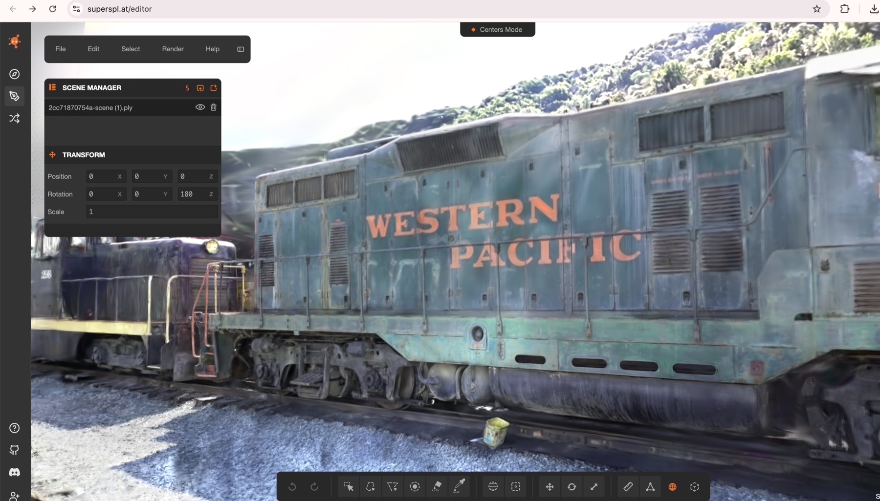
The per-scene means combine the pipeline setting with the subject being represented. Foliage, sky, distant background, reflections and occlusion change the rendering problem. A cross-scene score can describe each output, but it cannot isolate whether one budget or capture procedure was better. That is why the budget discussion above stays within one scene and still retains the end-to-end-run caveat.
PSNR is also only one view of quality. On playroom, the mean LPIPS moved from 0.293 at one million to 0.276 at four million while the mean paired-frame PSNR difference was -0.034 dB. I did not calculate paired uncertainty for LPIPS, so I treat that movement as descriptive. Final acceptance should include the views and visual defects relevant to the use case.
Compute and output created two different bills
Image count affected COLMAP most. Exhaustive matching compares every image pair, so its pair count grows quadratically. Across the measured jobs, matching ranged from roughly 17 to 29 milliseconds per pair. The same truck input measured 19.8 and 29.0 milliseconds per pair in two runs, a 46% increase. That is enough for capacity planning with a wide margin, not for a precise performance model.
Sequential matching is an obvious option for ordered video and could remove many unnecessary pairs. I estimated that alternative but did not run it, so it remains a design recommendation for the next version rather than a measured speedup.
Gaussian budget affected training, memory and artifact size:
| Truck budget | Training time | Sampled peak VRAM | USDZ size |
|---|---|---|---|
| 1 M | 12.9 min | 11,215 MiB | 236.1 MB |
| 3 M | 28.3 min | Not sampled reliably | 708.1 MB |
| 4 M | 35.2 min | 45,035 MiB | 944.1 MB |
The 4 M truck run used 97.8% of the L40S memory available to the process. The application sampled nvidia-smi every five seconds, so 45,035 MiB is a sampled peak and may miss a shorter spike. It shows that this run left little headroom on this card. It does not establish an exact four-million-Gaussian limit for every scene.
At the same one-million budget, playroom reached a sampled peak of 13,229 MiB, 18% above truck. Budget alone therefore cannot size a worker. Image dimensions and scene-specific training state also matter. An on-demand service should collect memory profiles from its own workload and route jobs with headroom rather than derive a fleet rule from the requested Gaussian count.
Artifact size was much more predictable in this exporter. USDZ grew by about 236.1 MB per million Gaussians and PLY by about 248.0 MB per million. The three- and four-million truck outputs differed by 0.008 dB across paired frames, while the larger job added about 236 MB to the USDZ and took seven more minutes to train. Storage, download and browser loading became part of the quality decision.
What these runs changed in ReconStudio
The budget comparisons exposed a limitation in the testbed: changing a trainer setting reran the entire pipeline. A cleaner comparison needs to fork a completed job after camera solving, preserve its selected frames, poses and held-out split, and vary only the trainer configuration.
I would add four pieces to the job record before treating ReconStudio as a stronger experiment system:
- Source and selected-frame checksums, plus a hash of the camera-solution artifact.
- The training seed, software revision and complete trainer configuration.
- A parent job identifier so a trainer-only fork carries explicit lineage.
- A comparison label that distinguishes a paired-frame observation from a repeated, isolated setting test.
The service path also becomes clearer. Camera-solve evidence can gate expensive training. Metric artifacts and their provenance stay part of the job contract. GPU workers can be selected from measured memory profiles, and artifact-size estimates can inform retention and download warnings before a job starts.
A convincing view can still hide bad bounds
The useful content occupied a small region of every exported cloud, while a few elongated Gaussians sat far away. On truck, the raw minimum-to-maximum bounding radius was about 720 times the radius calculated from the second to ninety-eighth percentiles. Train and playroom had still larger ratios.
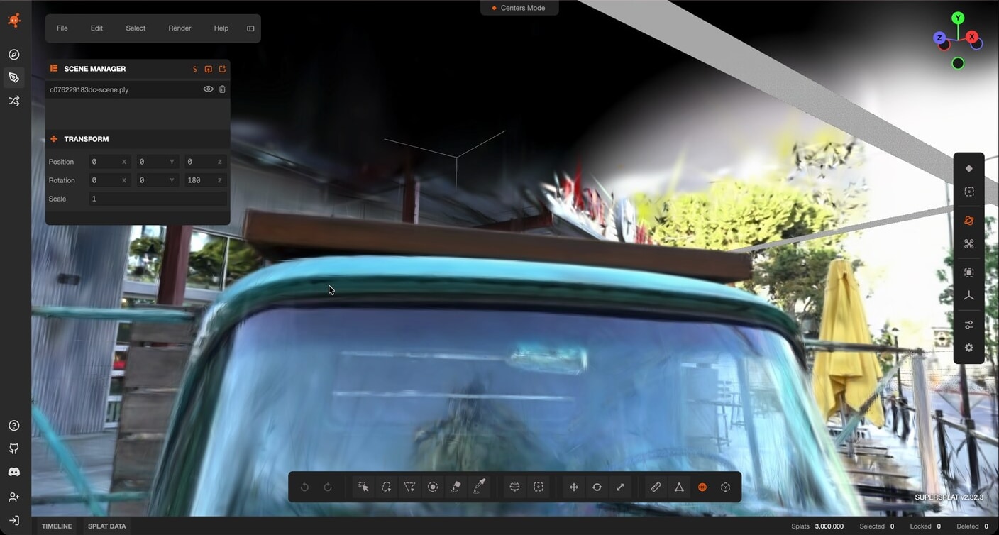
This is why an initial browser view can appear black or empty even when the asset is valid: fit-to-bounds may place the camera far from the useful content. Percentile bounds were a better default for framing. The artifacts also reinforced the representation boundary from Part 1: a visually strong splat still did not contain mesh surfaces, colliders, semantics or known physical scale.
What I would carry into the next run
I would use this sequence for a new scene:
- Verify the capture model first, including whether the images came from one camera, multiple physical cameras or a calibrated rig.
- Preserve the source artifacts and metric provenance. Missing, parsed and derived values need different states.
- Inspect feature count, registration, connected models and reprojection error together before spending time on training.
- Complete a credible baseline before comparing quality. For this run set, I use 30,000 iterations because the shorter end-to-end outputs were much worse.
- Fork from the same camera solution, preserve the held-out split, record the seed and repeat the setting when the decision matters. Paired frames alone do not capture run-to-run variation.
- Begin with a lower Gaussian budget and run one measured increase. Keep the increase when its gain matters for the use case.
- Sample memory on the target GPU and include output size in the decision. A model that barely trains or is awkward to distribute may be the wrong service output.
The experiment did not produce one setting for every reconstruction. It produced a repeatable workflow for finding the next setting to test, along with evidence that explains why a job succeeded or failed. It also showed what ReconStudio still needs before I can call its parameter comparisons controlled.
The code, setup notes, sample report and replay are in github.com/pr9868/reconstudio. Together, the fidelity article, the ReconStudio build and this run analysis cover the choice of representation, the service-shaped workflow and what happened when I exercised it.
Disclaimer: The views and opinions expressed in this account are those of my own and do not represent those of my employer, NVIDIA.